↜ Back to index Introduction to Numerical Analysis 2

Part b–Lecture 2

Conjugate gradient method

The conjugate gradient method (共役勾配法) is an iterative method (反復法) to find a solution of a linear system Ax = b when the n\times n matrix A is symmetric and positive definite. It is often abbreviated as CG method. Symmetric (対称) means that the transposed matrix (転置行列) is the same: A = A^t. A symmetric matrix is positive definite (正定値) if all its eigenvalues (固有値) are positive. Equivalently, if the following is satisfied: (Ax, x) > 0 \qquad \text{for all } x \neq 0. Here (\cdot, \cdot) is the inner product.

Example 1. The symmetric matrix \begin{pmatrix} 2 & 1\\ 1 & 2 \end{pmatrix} is positive definite because its eigenvalues are 1 and 3 and therefore both positive.

The matrix \begin{pmatrix} 2 & 3\\ 3 & 2 \end{pmatrix} is not positive definite as one of its eigenvalues is -1.

Example 2. A discretization of elliptic and parabolic partial differential equations by the finite difference method or the finite element method very often produces a linear system with a symmetric positive definite matrix.

The conjugate gradient method algorithm

We are given an n \times n matrix A and a n-dimensional vector b \in {{\mathbb{R}^{n}}} as an input. We also need to provide a tolerance \varepsilon > 0 that decides when the solution is “good enough” and we can stop.

It is an iterative method (反復法). We keep track of the current point x \in {{\mathbb{R}^{n}}} and the current search direction p \in {{\mathbb{R}^{n}}}. We also make use of other variables, most importantly the residual r = b - Ax \in {{\mathbb{R}^{n}}}. The norm of r, \|r\| := \sqrt{r_1^2 + r_2^2 + \cdots + r_n^2} = \sqrt{(r, r)}, tells us how good the current point is as a solution of the system Ax = b since we want to find x that gives r = 0. Because we usually only need an approximate solution with certain accuracy, we stop when \|r\| < \varepsilon. We store the value \|r\|^2 = (r, r) in a variable \rho \in {\mathbb{R}}, and its previous value in a variable \rho_{\rm old} \in {\mathbb{R}}.

Here is the algorithm:

x \leftarrow 0
r \leftarrow b
\rho \leftarrow (r, r)
p \leftarrow r
For k = 1, 2, …, n do
- \alpha \leftarrow \frac{\rho}{(A p, p)}
- x \leftarrow x + \alpha p
- r \leftarrow r - \alpha Ap
- \rho_{\rm old} \leftarrow \rho
- \rho \leftarrow (r, r)
- If \sqrt{\rho} < \varepsilon, exit the loop
- p \leftarrow r + \frac{\rho}{\rho_{\rm old}} p
- Repeat for next k.
Return x as the result

In Fortran code, x, r, p are stored as real one-dimensional arrays, and \rho, \rho_{\rm old} and \alpha are real variables.

Exercise 1. Find the number of multiplications of real numbers that the algorithm has to perform in each iteration of the loop. It should be a function of n.

Notes on the implementation in Fortran

In the implementation, we can use the functions inner and mv_mul that we implemented in Lecture 1.
The most time-consuming operation in the above algorithm is the matrix-vector multiplication Ap. To not have to perform it twice in each iteration, it is a good idea to store the result in a variable.

Motivation

Symmetric positive definite matrices are invertible (正則) and have the nice property that the function f(x) := \frac12 (Ax, x) - (b,x), \qquad x \in {\mathbb{R}}^n, is a convex quadratic function of n variables x_1, x_2, …, x_n with a single global minimum exactly at A^{-1} b. So if we find the point of minimum of f, we have solved Ax = b. Here I use the notation (\cdot, \cdot) for the inner product on {\mathbb{R}}^n.

Example 3. Given matrix A = \begin{pmatrix} 2 & 1\\ 1 & 2 \end{pmatrix} and vector b = (5, 1), the function f is f(x) = f(x_1, x_2) = x_1^2 + x_1x_2 + x_2^2 - 5x_1 - 1x_2.

If x is a point of minimum of f, we must have \frac{\partial f}{\partial x_1} (x) = 0 and \frac{\partial f}{\partial x_2} (x) = 0 (that is, \nabla f(x) = 0). After a simple calculation we recover the two equations A x = b.

Exercise 2. Plot the function f from the previous exercise using gnuplot (command splot). Verify that the minimum of the function occurs at the point x that solves Ax = b.

You might find the following gnuplot commands useful:

set isosamples 21           # increase the resolution of the plot
set contour both            # plot contour lines both on the graph and the base
set cntrparam levels 10     # set the number of contour lines to 10

This fact is what motivates the conjugate gradient method:

We start from an initial guess of a solution, x^{(0)}, for example x^{(0)} = 0. Then we iteratively produce a sequence of points x^{(1)}, x^{(2)}, …, so that the value of f(x^{(k)} decreases, and in the end they converge to the point of minimum A^{-1} b of f.

The simplest way is to move the current point in the direction in which f is decreasing the fastest. This is the direction opposite to the gradient of f at the current point, -\nabla f(x^{(k)}). This yields the gradient descent method (最急降下法). Conjugate gradient method is an improvement of this method by adjusting the direction in which we move x^{(k)} to produce x^{(k+1)}.

If you want to learn more, see the wikipedia article.

Exercises

Exercise 3. Implement the conjugate gradient algorithm in Fortran and do the following:

First make sure that your program works with the following A and x:

integer, parameter :: n = 3
real a(n, n), b(n)

a(1,:) = [2., -1., 0.]
a(2,:) = [-1., 2., -1.]
a(3,:) = [0., -1., 2.]

b = [1., 1., 1.]

The output of my code is:

 Iteration            0
     x =    0.00000000       0.00000000       0.00000000    
     r =    1.00000000       1.00000000       1.00000000    

 Iteration            1
     x =    1.50000000       1.50000000       1.50000000    
     r =  -0.500000000       1.00000000     -0.500000000    

 Solution
     x =    1.50000000       2.00000000       1.50000000    
     r =    0.00000000       0.00000000       0.00000000

Then modify the code so that the program reads a positive integer n and a real number \gamma, and runs the conjugate gradient algorithm for the matrix A_{ij} := \begin{cases} \gamma, & i =j,\\ -1, & |i - j| = 1,\\ 0 & \text{otherwise}, \end{cases} and vector b with b_i = 1 for all i.

Note that with \gamma = 2 and n = 3 this is the matrix in 1.

Use {\varepsilon}= 10^{-6}.

For each iteration print the iteration number and the Euclidean norm \|r\| of r after the update in the form
```
       1   1.40998209
       2  0.470300049
       3  0.176379248
       4   6.71928748E-02
       ...
```
Run the computation for
- n = 1000, \gamma = 3
- n = 1000, \gamma = 2
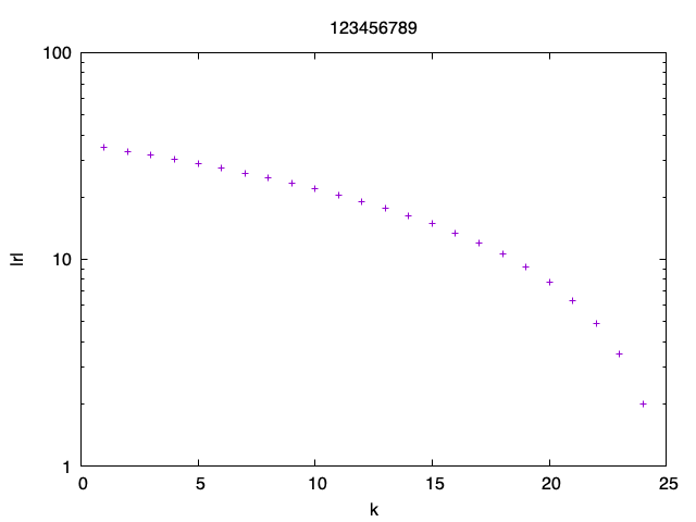
In each case, plot the graph of the norm of r as a function of the iteration number in gnuplot.

Since the norm of the residual varies over multiple orders, you can use the logarithmic scale for the vertical axis to improve the readability by running the gnuplot command:
```
set logscale y
```
Submit both plots as images to LMS. As the plot title use your student ID number.

Example. This is how the plot looks like for n = 50 and \gamma = 2
Save the solution x for n = 100 and \gamma = 2 into a file and plot the values using gnuplot. Submit the image file to LMS. As the title use your student ID number.

Exercise 4. Here are some more diagonal matrices to try. In the following we always take A_{ij} = 0 if i \neq j.

Try the CG method for the diagonal matrix A with entries A_{ii} = i and A_{ij} = 0 for i \neq j. Use b = (1, 1, \ldots, 1). Try n = 1000.

Plot the graph of the norm of the residual r as in the previous exercise.
Instead set A_{ii} = 2 for all i. How many steps does the method need to find the solution?
How about a matrix with A_{ii} = 1 if i < n/2 and A_{ii} = 100 otherwise?

Exercise 5. Implement the conjugate gradient algorithm as a Fortran function cg that takes A, b and \varepsilon as 3 arguments and returns the solution x. The function cg should not modify the input arguments.

The function definition can look something like

function cg(a, b, eps) result(x)
    real a(:,:), b(:), eps, x(size(b))
    ...
end

Hints. You can return from a function early by using the return command.

Advantages of the conjugate gradient method

The algorithm is very simple to implement.
It can be proved that the algorithm will converge to the exact solution in at most n steps where n is the size of the matrix (if there are no rounding errors). But in practice for “good” matrices¹ or with some improvements like preconditioning (前処理), we get a very good approximate solution for a much smaller number of steps than n. We will discuss preconditioning in the coming lectures.
The most time-consuming step is the matrix-vector multiplication Ap. For a general matrix, this requires on the order of n^2 operations. However, in practice (for example, when solving partial differential equations numerically), the matrix A is often sparse (疎行列): there are only very few nonzero entries in each row, so the number of operations required to compute Ap is proportional to the number of nonzero elements in A.

We also do not need to store all n^2 elements of the sparse matrix. It is enough to store the nonzero elements (and their positions). We will learn how to take advantage of sparse matrices later in the course. This way it is possible to handle matrices with sizes 10^6 \times 10^6 and bigger and find the solution of systems of millions of equations relatively quickly.

In contrast, for the Gaussian elimination or the LU decomposition we almost always have to store n^2 elements, even if the matrix is sparse.²

A “good” matrix here means a matrix with a small condition number (条件数), the size of the ratio between the largest eigenvalue and the smallest eigenvalue.↩︎
There are some important exceptions like the tridiagonal matrix when the Gaussian elimination is very efficient.↩︎