Numerics for the two-phase Stefan problem

Introduction

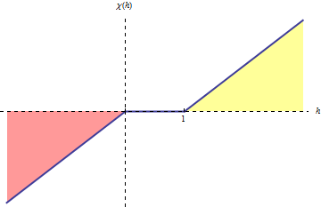
The following videos show the evolution of enthalpy $h$ in the two-phase Stefan problem with no-flux boundary in 2D: $$\begin{cases} h_t(x,t) - \Delta \chi(h(x,t)) = f(x,t), & \text{in } \Omega \times (0, T)\\ \frac{\partial \chi(u)}{\nu} = 0, & \text{on } \partial \Omega \times (0,T)\\ h(x,0) = h_0(x), \end{cases}$$ where $h$ is the enthalpy, $f$ is the volumetric heat source and $\chi(h)$ is the temperature. The function $\chi$ is defined as $$\chi(s) = \min(s, \max(0, s -1)) = \begin{cases} s & s < 0,\\ 0 & 0 \leq s \leq 1 & s-1 & s > 1, \end{cases}$$ see figure 1.

The solutions contain the following regions:

• solid – red
• liquid – yellow
• mushy region – blue

Images were produced using Mathematica 7 and encoded using mencoder. To view these videos, you need to be able to play videos from youtube.

Videos